PnsPy documentation#
Module reference#
Principal nested spheres (PNS) analysis [1].
Jung, Sungkyu, Ian L. Dryden, and James Stephen Marron. “Analysis of principal nested spheres.” Biometrika 99.3 (2012): 551-568.
- pns.pns(x, n_components, tol=0.001, maxiter=None, lm_kwargs=None)[source]#
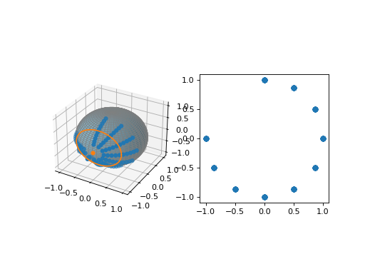
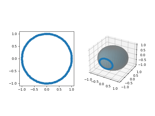
Principal nested spheres analysis.
- Parameters:
- xreal array of shape (N, d+1)
Data on a d-sphere.
- n_componentsint
Target dimension.
- tolfloat, default=1e-3
Convergence tolerance in radians.
- maxiterint, optional
Maximum number of iterations for the optimization. If None, the number of iterations is not checked.
- lm_kwargsdict, optional
Additional keyword arguments to be passed for Levenberg-Marquardt optimization. Passed to
pns.pss().
- Returns:
- vslist of array
Principal axes.
- rs1-D array of length (d+1-n_components)
Principal geodesic distances.
- xis2-D array of shape (N, d+1-n_components)
Unscaled residuals.
- x_transformreal array of shape (N, n_components)
Data transformed onto low-dimensional sphere.
Notes
The input data is \(x \in S^d \subset \mathbb{R}^{d+1}\).
The \(k\)-th element of vs, rs and xis are:
The principal axis \(\hat{v}_{k} \in S^{d-k+1} \subset \mathbb{R}^{d-k+2}\),
The principal geodesic distance \(\hat{r}_k \in \mathbb{R}\), and
Unscaled residual \(\xi_{d-k}\).
Examples
>>> from pns import pns
>>> from pns.util import unit_sphere, circular_data, circle_3d
>>> x = circular_data([0, -1, 0])
>>> vs, rs, _, x_transform = pns(x, 2)
>>> import matplotlib.pyplot as plt
... fig = plt.figure()
... ax1 = fig.add_subplot(121, projection='3d', computed_zorder=False)
... ax1.plot_surface(*unit_sphere(), color='skyblue', alpha=0.6, edgecolor='gray')
... ax1.scatter(*x.T)
... ax1.scatter(*vs[0])
... ax1.plot(*circle_3d(vs[0], rs[0]), color="tab:orange", zorder=10)
... ax2 = fig.add_subplot(122)
... ax2.scatter(*x_transform.T)
... ax2.set_aspect("equal")
- pns.fit_transform(X, n_components, type='intrinsic', tol=0.001, maxiter=None, lm_kwargs=None)[source]#
Fit PNS and transform data into low-dimensional hypersphere.
- Parameters:
- Xreal array of shape (N, d+1)
Extrinsic coordinates of data on a
d-dimensional hypersphere, embedded in ad+1-dimensional space.- n_componentsint
Target dimension.
- type{‘intrinsic’, ‘extrinsic’}
Type of the output coordinates.
- tolfloat, default=1e-3
Convergence tolerance in radians.
- maxiterint, optional
Maximum number of iterations for the optimization. If None, the number of iterations is not checked.
- lm_kwargsdict, optional
Additional keyword arguments to be passed for Levenberg-Marquardt optimization. Passed to
pns.pns().
- Returns:
- vslist of array
Principal axes.
- rs1-D array of length (d+1-n_components)
Principal geodesic distances.
- X_transformarray of shape (N, n_components)
Coordinates of transformed data on a low-dimensional unit hypersphere.
Examples
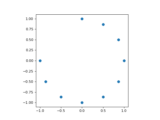
Extrinsic transformation:
>>> from pns import fit_transform
>>> from pns.util import circular_data
>>> x = circular_data([0, -1, 0])
>>> _, _, x_transformed = fit_transform(x, n_components=2, type='extrinsic')
>>> import matplotlib.pyplot as plt
... plt.scatter(*x_transformed.T)
... plt.gca().set_aspect("equal")
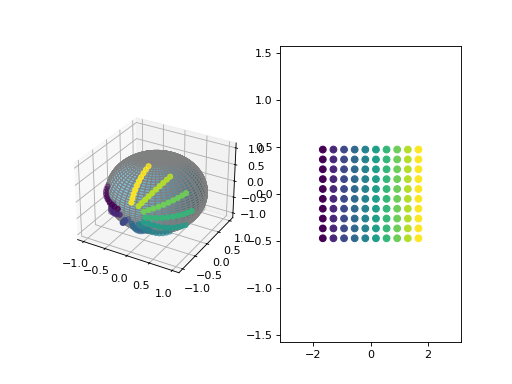
Intrinsic transformation:
>>> import numpy as np
>>> from pns.util import unit_sphere
>>> _, _, x_transformed = fit_transform(x, n_components=2, type='intrinsic')
>>> fig = plt.figure()
... ax1 = fig.add_subplot(121, projection='3d', computed_zorder=False)
... ax1.plot_surface(*unit_sphere(), color='skyblue', edgecolor='gray')
... ax1.scatter(*x.T, c=x_transformed[:, 0])
... ax2 = fig.add_subplot(122)
... ax2.scatter(*x_transformed.T, c=x_transformed[:, 0])
... ax2.set_xlim(-np.pi, np.pi)
... ax2.set_ylim(-np.pi/2, np.pi/2)


- pns.transform(X, vs, rs, n_components, type='intrinsic')[source]#
Transform data using the fitted PNS.
- Parameters:
- X(N, d+1) real array
Extrinsic coordinates of data on a
d-dimensional hypersphere, embedded in ad+1-dimensional space.- vslist of k real arrays
Subsphere axes.
- rslist of k scalars
Subsphere geodesic distances.
- n_componentsint
Target dimension.
- type{‘intrinsic’, ‘extrinsic’}
Type of the output coordinates.
- Returns:
- (N, n_components) real array
Coordinates of transformed data on a low-dimensional unit hypersphere.
Notes
If type is
intrinsic,kmust bed. If type isextrinsic,kmust be at leastd + 1 - n_components.Examples
Extrinsic transformation:
>>> from pns import fit_transform, transform
>>> from pns.util import circular_data
>>> x = circular_data([0, -1, 0])
>>> vs, rs, _ = fit_transform(x, n_components=2, type='extrinsic')
>>> x_transformed = transform(x, vs, rs, n_components=2, type='extrinsic')
>>> import matplotlib.pyplot as plt
... plt.scatter(*x_transformed.T)
... plt.gca().set_aspect("equal")
Intrinsic transformation:
>>> import numpy as np
>>> from pns.util import unit_sphere
>>> vs, rs, _ = fit_transform(x, n_components=2, type='intrinsic')
>>> x_transformed = transform(x, vs, rs, n_components=2, type='intrinsic')
>>> fig = plt.figure()
... ax1 = fig.add_subplot(121, projection='3d', computed_zorder=False)
... ax1.plot_surface(*unit_sphere(), color='skyblue', edgecolor='gray')
... ax1.scatter(*x.T, c=x_transformed[:, 0])
... ax2 = fig.add_subplot(122)
... ax2.scatter(*x_transformed.T, c=x_transformed[:, 0])
... ax2.set_xlim(-np.pi, np.pi)
... ax2.set_ylim(-np.pi/2, np.pi/2)
- pns.inverse_transform(X, vs, rs, type='intrinsic')[source]#
Inverse-transform data using the fitted PNS.
- Parameters:
- X(N, n_components) real array
Coordinates of transformed data on a low-dimensional unit hypersphere.
- vslist of k real arrays
Subsphere axes.
- rslist of k scalars
Subsphere geodesic distances.
- type{‘intrinsic’, ‘extrinsic’}
Type of the output coordinates.
- Returns:
- (N, d+1) real array
Extrinsic coordinates of data on a
d-dimensional hypersphere, embedded in ad+1-dimensional space.
Notes
If type is
intrinsic,kmust bed. If type isextrinsic,kmust be at leastd + 1 - n_components.Examples
Extrinsic transformation:
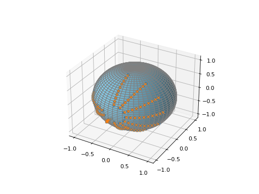
>>> from pns import fit_transform, inverse_transform
>>> from pns.util import circular_data, unit_sphere
>>> x = circular_data([0, -1, 0])
>>> vs, rs, x_transformed = fit_transform(x, n_components=2, type='extrinsic')
>>> x_reconstructed = inverse_transform(x_transformed, vs, rs, type='extrinsic')
>>> import matplotlib.pyplot as plt
... fig = plt.figure()
... ax = fig.add_subplot(projection='3d', computed_zorder=False)
... ax.plot_surface(*unit_sphere(), color='skyblue', alpha=0.6, edgecolor='gray')
... ax.scatter(*x.T, marker=".", zorder=10)
... ax.scatter(*x_reconstructed.T, marker="x", zorder=10)
Intrinsic transformation:
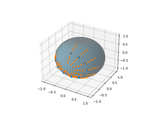
>>> vs, rs, x_transformed = fit_transform(x, n_components=2, type='intrinsic')
>>> x_reconstructed = inverse_transform(x_transformed, vs, rs, type='intrinsic')
>>> import matplotlib.pyplot as plt
... ax = plt.figure().add_subplot(projection='3d', computed_zorder=False)
... ax.plot_surface(*unit_sphere(), color='skyblue', edgecolor='gray')
... ax.scatter(*x.T, marker="o", zorder=10)
... ax.scatter(*x_reconstructed.T, marker="x", zorder=10)
Data transformation#
Classes to transform data on a hypersphere.
- pns.transformers.project(x, v, r)[source]#
Minimum-geodesic projection of points to a subsphere.
- Parameters:
- x(N, m+1) real array
Extrinsic coordinates of data on a
d-dimensional hypersphere, embedded in ad+1-dimensional space.- v(m+1,) real array
Subsphere axis.
- rscalar
Subsphere geodesic distance.
- Returns:
- xP(N, m+1) real array
Extrinsic coordinates of data on a
d-dimensional hypersphere, projected onto the found principal subsphere.- res(N, 1) real array
Projection residuals.
Notes
This is the function \(P: S^{d-k+1} \to A_{d-k}(v_k, r_k ) \subset S^{d-k+1}\) for \(k = 1, 2, \ldots, d\) in the original paper. Here, \(A_{d-k}(v_k, r_k)\) is a subsphere of the hypersphere \(S^{d-k+1}\). The input and output data dimension are \(m+1\), where \(m = d-k+1\).
The resulting points have same number of components but their rank is reduced by one in the manifold.
Examples
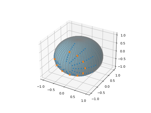
>>> from pns.pss import pss
>>> from pns.transformers import project
>>> from pns.util import unit_sphere, circular_data
>>> x = circular_data([0, -1, 0]).reshape(-1, 3)
>>> v, r = pss(x)
>>> A, _ = project(x, v, r)
>>> import matplotlib.pyplot as plt
... ax = plt.figure().add_subplot(projection='3d', computed_zorder=False)
... ax.plot_surface(*unit_sphere(), color='skyblue', alpha=0.6, edgecolor='gray')
... ax.scatter(*x.T, marker="x")
... ax.scatter(*A.T, marker=".")

- pns.transformers.inverse_project(xP, res, v, r)[source]#
Inverse of
project().- Parameters:
- xP(N, m+1) real array
Extrinsic coordinates of data on a
d-dimensional hypersphere, projected onto the found principal subsphere.- res(N, 1) real array
Projection residuals.
- v(m+1,) real array
Subsphere axis.
- rscalar
Subsphere geodesic distance.
- Returns:
- x(N, m+1) real array
Extrinsic coordinates of data on a
d-dimensional hypersphere, embedded in ad+1-dimensional space.
Examples
>>> from pns.pss import pss
>>> from pns.transformers import project, inverse_project
>>> from pns.util import unit_sphere, circular_data
>>> x = circular_data([0, -1, 0])
>>> v, r = pss(x)
>>> xP, res = project(x, v, r)
>>> x_invprj = inverse_project(xP, res, v, r)
>>> import matplotlib.pyplot as plt
... ax = plt.figure().add_subplot(projection='3d', computed_zorder=False)
... ax.plot_surface(*unit_sphere(), color='skyblue', alpha=0.6, edgecolor='gray')
... ax.scatter(*xP.T, marker="x", zorder=10)
... ax.scatter(*x_invprj.T, marker=".")
- pns.transformers.embed(x, v, r)[source]#
Embed data on a sub-hypersphere to a low-dimensional unit hypersphere.
- Parameters:
- x(N, m+1) real array
Data \(x \in A_{m-1} \subset S^m \subset \mathbb{R}^{m+1}\), on a subsphere \(A_{m-1}\) of a unit hypersphere \(S^m\).
- v(m+1,) real array
Sub-hypersphere axis.
- rscalar
Sub-hypersphere geodesic distance.
- Returns:
- (N, m) real array
Data \(x^\dagger\) on a low-dimensional unit hypersphere \(S^{m-1}\).
Notes
This is the function \(f_k: A_{d-k}(v_k, r_k) \subset S^{d-k+1} \to S^{d-k}\) for \(k = 1, 2, \ldots, d-1\) in the original paper. Here, \(A_{d-k}(v_k, r_k)\) is a subsphere of the hypersphere \(S^{d-k+1}\). The input is \(x \in S^m \subset \mathbb{R}^{m+1}\) and the output is \(x^\dagger \in S^{m-1} \subset \mathbb{R}^{m}\), where \(m = d-k+1\).
Examples
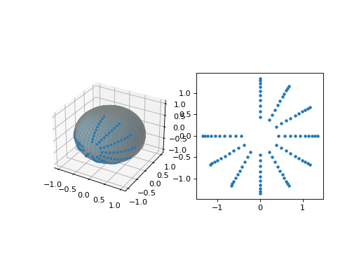
>>> from pns.pss import pss
>>> from pns.transformers import embed
>>> from pns.util import unit_sphere, circular_data
>>> x = circular_data([0, -1, 0])
>>> v, r = pss(x)
>>> x_embed = embed(x, v, r)
>>> import matplotlib.pyplot as plt
... fig = plt.figure()
... ax1 = fig.add_subplot(121, projection='3d', computed_zorder=False)
... ax1.plot_surface(*unit_sphere(), color='skyblue', alpha=0.6, edgecolor='gray')
... ax1.scatter(*x.T, marker=".", zorder=10)
... ax2 = fig.add_subplot(122)
... ax2.scatter(*x_embed.T, marker=".", zorder=10)
... ax2.set_aspect("equal")
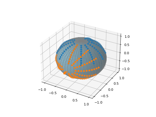
- pns.transformers.reconstruct(x, v, r)[source]#
Reconstruct data on a low-dimensional unit hypersphere. to a sub-hypersphere.
- Parameters:
- x(N, m) real array
Data \(x^\dagger\) on a low-dimensional unit hypersphere \(S^{m-1}\).
- v(m+1,) real array
Sub-hypersphere axis.
- rscalar
Sub-hypersphere geodesic distance.
- Returns:
- (N, m+1) real array
Data \(x \in A_{m-1} \subset S^m \subset \mathbb{R}^{m+1}\), on a subsphere \(A_{m-1}\) of a unit hypersphere \(S^m\).
Notes
This is the function \(f^{-1}_k: S^{d-k} \to A_{d-k}(v_k, r_k) \subset S^{d-k+1}\) for \(k = 1, 2, \ldots, d-1\) in the original paper. Here, \(A_{d-k}(v_k, r_k)\) is a subsphere of the hypersphere \(S^{d-k+1}\). The input is \(x^\dagger \in S^{m-1} \subset \mathbb{R}^{m}\) and the output is \(x \in S^m \subset \mathbb{R}^{m+1}\), where \(m = d-k+1\).
Examples
>>> import numpy as np
>>> from pns.transformers import reconstruct
>>> from pns.util import unit_sphere
>>> t = np.linspace(0, 2 * np.pi, 100)
>>> x = np.vstack((np.cos(t), np.sin(t))).T
>>> x_rec = reconstruct(x, np.array([0, -1, 0]), 0.5)
>>> import matplotlib.pyplot as plt
... fig = plt.figure()
... ax1 = fig.add_subplot(121)
... ax1.scatter(*x.T)
... ax1.set_aspect("equal")
... ax2 = fig.add_subplot(122, projection='3d', computed_zorder=False)
... ax2.plot_surface(*unit_sphere(), color='skyblue', alpha=0.6, edgecolor='gray')
... ax2.scatter(*x_rec.T)
PSS detection#
Detect the principal subsphere by optimization.
- pns.pss.pss(x, tol=0.001, maxiter=None, lm_kwargs=None)[source]#
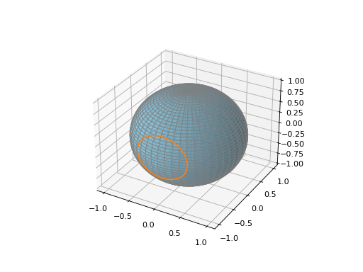
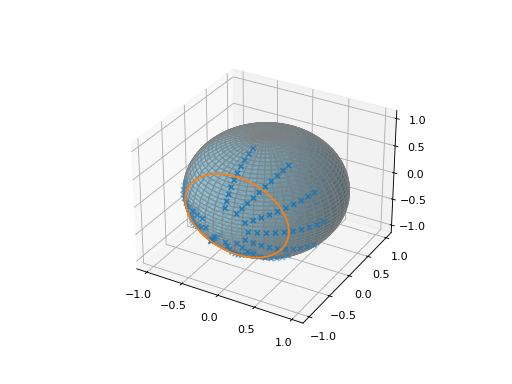
Find the principal subsphere (PSS) from data on a hypersphere.
- Parameters:
- x(N, d+1) real array
Extrinsic coordinates of data on a
d-dimensional hypersphere, embedded in ad+1-dimensional space.- tolfloat, default=1e-3
Convergence tolerance in radian.
- maxiterint, optional
Maximum number of iterations for the optimization. If None, the number of iterations is not checked.
- lm_kwargsdict, optional
Additional keyword arguments to be passed for Levenberg-Marquardt optimization. Follows the signature of
scipy.optimize.least_squares().
- Returns:
- v(d+1,) real array
Estimated principal axis of the subsphere in extrinsic coordinates.
- rscalar in [0, pi]
Geodesic distance from the pole by v to the estimated principal subsphere.
Notes
This function determines the best fitting subsphere \(\hat{A}_{d-k} = A_{d-k}(\hat{v}_k, \hat{r}_k) \subset S^{d-k+1}\) for \(k = 1, 2, \ldots, d\).
The Fréchet mean \(\hat{A}_0\) of the lowest level best fitting subsphere \(\hat{A}_1\) is also determined by this function.
Examples
>>> from pns.pss import pss
>>> from pns.util import unit_sphere, circular_data, circle_3d
>>> x = circular_data([0, -1, 0])
>>> v, r = pss(x)
>>> import matplotlib.pyplot as plt
... ax = plt.figure().add_subplot(projection='3d', computed_zorder=False)
... ax.plot_surface(*unit_sphere(), color='skyblue', alpha=0.6, edgecolor='gray')
... ax.scatter(*x.T, marker="x")
... ax.plot(*circle_3d(v, r), color="tab:orange", zorder=10)
Hypersphere functions#
Basic functions to handle data on a hypersphere.
- Conventions for intrinsic coordiates are:
xi[…, 0]: azimuthal angle in [-pi, pi]
xi[…, 1:]: centered elevation angles in [-pi/2, pi/2]
- pns.base.intrinsic_to_extrinsic(xi)[source]#
Convert hypersphere intrinsic coordinates to extrinsic.
- Parameters:
- xiarray of shape (N, d)
Hyperspherical coordinates.
- Returns:
- Xarray of shape (N, d+1)
Cartesian coordinates.
Notes
- Intrinsic coordiates are:
xi[…, 0]: azimuthal angle in [-pi, pi]
xi[…, 1:]: centered elevation angles in [-pi/2, pi/2]
Examples
>>> import numpy as np
>>> from pns.base import intrinsic_to_extrinsic
>>> xi = np.array([[0, np.pi/2]])
>>> X = intrinsic_to_extrinsic(xi)
>>> np.isclose(X, [[0, 0, 1]])
array([[ True,  True,  True]])
- pns.base.extrinsic_to_intrinsic(X)[source]#
Convert hypersphere extrinsic coordinates to intrinsic.
- Parameters:
- Xarray of shape (N, d+1)
Cartesian coordinates.
- Returns:
- xiarray of shape (N, d)
Hyperspherical coordinates.
Examples
>>> from pns.base import extrinsic_to_intrinsic
>>> from pns.util import circular_data
>>> X = circular_data()
>>> X.shape
(100, 3)
>>> extrinsic_to_intrinsic(X).shape
(100, 2)
- pns.base.rotation_matrix(v)[source]#
Rotation matrix.
Moves \(v\) to the north pole.
- Parameters:
- v(m+1) real array
Unit-norm direction vector.
- Returns:
- (m+1, m+1) array of float64
Rotational matrix.
Notes
This is the function \(R(v_k)\) in the original paper.
Examples
Moving
[0, 1, 0]to the north pole, in other words, moving the north pole to[0, -1, 0].>>> from pns.base import rotation_matrix >>> from pns.util import unit_sphere, circular_data >>> X = circular_data() >>> R = rotation_matrix([0, 1, 0]) >>> X_rotated = X @ R.T >>> import matplotlib.pyplot as plt ... ax = plt.figure().add_subplot(projection='3d', computed_zorder=False) ... ax.plot_surface(*unit_sphere(), color='skyblue', alpha=0.6, edgecolor='gray') ... ax.scatter(*X.T) ... ax.scatter(*X_rotated.T)
- pns.base.exp_map(z)[source]#
Exponential map of hypersphere at (0, 0, …, 0, 1).
- Parameters:
- z(N, d) real array
Vectors on tangent space.
- Returns:
- (N, d+1) real array
Points on d-sphere.
- pns.base.log_map(x)[source]#
Log map of hypersphere at (0, 0, …, 0, 1).
- Parameters:
- x(N, d+1) real array
Points on d-sphere.
- Returns:
- (N, d) real array
Vectors on tangent space.
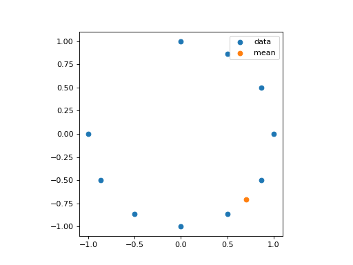
- pns.base.circle_mean(X)[source]#
Frechet mean of data on a circle.
- Parameters:
- Xreal array of shape (N, 2)
- Returns:
- meanarray of shape (2,)
Notes
Uses the algorithm [1] implemented by the Geomstats [2] package.
Copyright (c) 2018 Nina Miolane
References
[1]Hotz, T. and S. F. Huckemann (2015), “Intrinsic means on the circle: Uniqueness, locus and asymptotics”, Annals of the Institute of Statistical Mathematics 67 (1), 177-193. https://arxiv.org/abs/1108.2141
Examples
>>> import numpy as np
>>> from pns.base import circle_mean
>>> t = np.linspace(-np.pi, np.pi / 2, 10)
>>> X = np.stack([np.cos(t), np.sin(t)]).T
>>> mean = circle_mean(X)
>>> import matplotlib.pyplot as plt
... plt.scatter(*X.T, label="data")
... plt.scatter(*mean, label="mean")
... plt.legend()
... plt.gca().set_aspect("equal")
Utilities#
Utility functions to generate and plot sample data.
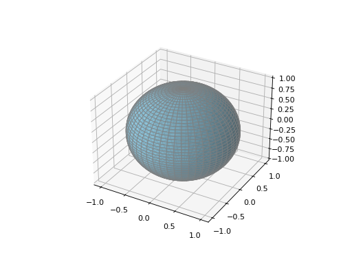
- pns.util.unit_sphere()[source]#
Helper function to plot a unit sphere.
- Returns:
- x, y, zarray
Coordinates for unit sphere.
Examples
>>> from pns.util import unit_sphere
>>> import matplotlib.pyplot as plt
... ax = plt.figure().add_subplot(projection='3d')
... ax.plot_surface(*unit_sphere(), color='skyblue', alpha=0.6, edgecolor='gray')
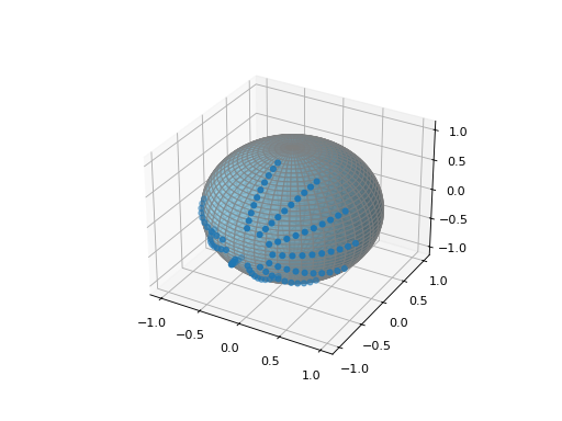
- pns.util.circular_data(v=(0, 0, 1))[source]#
Circular data on a 3D unit sphere.
- Parameters:
- varray of shape (3,), default=(0, 0, 1)
Unit vector to center of circle.
- Returns:
- ndarray of shape (100, 3)
Data coordinates.
Examples
>>> from pns.util import unit_sphere, circular_data
>>> v = [0, -1, 0]
>>> X = circular_data(v)
>>> X.shape
(100, 3)
>>> import matplotlib.pyplot as plt
... ax = plt.figure().add_subplot(projection='3d', computed_zorder=False)
... ax.plot_surface(*unit_sphere(), color='skyblue', alpha=0.6, edgecolor='gray')
... ax.scatter(*X.T)
- pns.util.circle_3d(v, theta, n=100)[source]#
Helper function to plot a circle in 3D.
- Parameters:
- v(3,) array
Unit vector to center of circle in 3D.
- thetascalar
Geodesic distance.
- nint, default=100
Number of points.
Examples
>>> from pns.util import unit_sphere, circle_3d
>>> circle = circle_3d([0, -1, 0], 0.5)
>>> import matplotlib.pyplot as plt
... ax = plt.figure().add_subplot(projection='3d')
... ax.plot_surface(*unit_sphere(), color='skyblue', alpha=0.6, edgecolor='gray')
... ax.plot(*circle, color="tab:orange", zorder=10)